Code example: Wiener filter#

Introduction#

IFT starting point:

d = Rs+n

Typically, $s$ is a continuous field, $d$ a discrete data vector. Particularly, $R$ is not invertible.

IFT aims at inverting the above uninvertible problem in the best possible way using Bayesian statistics.

NIFTy (Numerical Information Field Theory) is a Python framework in which IFT problems can be tackled easily.

Main Interfaces:

Spaces: Cartesian, 2-Spheres (Healpix, Gauss-Legendre) and their respective harmonic spaces.
Fields: Defined on spaces.
Operators: Acting on fields.

Wiener filter on one-dimensional fields#

Assumptions#

$d=Rs+n$ , $R$ linear operator.
$\mathcal P (s) = \mathcal G (s,S)$ , $\mathcal P (n) = \mathcal G (n,N)$ where $S, N$ are positive definite matrices.

Posterior#

The Posterior is given by:

$\mathcal P (s|d) \propto P(s,d) = \mathcal G(d-Rs,N) \,\mathcal G(s,S) \propto \mathcal G (s-m,D)$

where $ $m = Dj$ $with$ $D = (S^{-1} +R^\dagger N^{-1} R)^{-1} , \quad j = R^\dagger N^{-1} d.$ $

Let us implement this in NIFTy!

In NIFTy#

We assume statistical homogeneity and isotropy. Therefore the signal covariance $S$ is diagonal in harmonic space, and is described by a one-dimensional power spectrum, assumed here as $ $P(k) = P_0\,\left(1+\left(\frac{k}{k_0}\right)^2\right)^{-\gamma /2},$ $with$ P_0 = 0.2, k_0 = 5, \gamma = 4$.
$N = 0.2 \cdot \mathbb{1}$ .
Number of data points $N_{pix} = 512$ .
reconstruction in harmonic space.
Response operator: $ $R = FFT_{\text{harmonic} \rightarrow \text{position}}$ $

N_pixels = 512     # Number of pixels

def pow_spec(k):
    P0, k0, gamma = [.2, 5, 4]
    return P0 / ((1. + (k/k0)**2)**(gamma / 2))

Implementation#

Import Modules#

%matplotlib inline
import numpy as np
import nifty8 as ift
import matplotlib.pyplot as plt

plt.rcParams['figure.dpi'] = 100

Implement Propagator#

def Curvature(R, N, Sh):
    IC = ift.GradientNormController(iteration_limit=50000,
                                    tol_abs_gradnorm=0.1)
    # WienerFilterCurvature is (R.adjoint*N.inverse*R + Sh.inverse) plus some handy
    # helper methods.
    return ift.WienerFilterCurvature(R,N,Sh,iteration_controller=IC,iteration_controller_sampling=IC)

Conjugate Gradient Preconditioning#

$D$ is defined via: $ $D^{-1} = \mathcal S_h^{-1} + R^\dagger N^{-1} R.$ $In the end, we want to apply$ D $to$ j $, i.e. we need the inverse action of$ D^{-1}$. This is done numerically (algorithm: Conjugate Gradient).

Generate Mock data#

Generate a field $s$ and $n$ with given covariances.
Calculate $d$ .

s_space = ift.RGSpace(N_pixels)
h_space = s_space.get_default_codomain()
HT = ift.HarmonicTransformOperator(h_space, target=s_space)

# Operators
Sh = ift.create_power_operator(h_space, power_spectrum=pow_spec, sampling_dtype=float)
R = HT # @ ift.create_harmonic_smoothing_operator((h_space,), 0, 0.02)

# Fields and data
sh = Sh.draw_sample()
noiseless_data=R(sh)
noise_amplitude = np.sqrt(0.2)
N = ift.ScalingOperator(s_space, noise_amplitude**2, float)

n = ift.Field.from_random(domain=s_space, random_type='normal',
                          std=noise_amplitude, mean=0)
d = noiseless_data + n
j = R.adjoint_times(N.inverse_times(d))
curv = Curvature(R=R, N=N, Sh=Sh)
D = curv.inverse

Run Wiener Filter#

m = D(j)

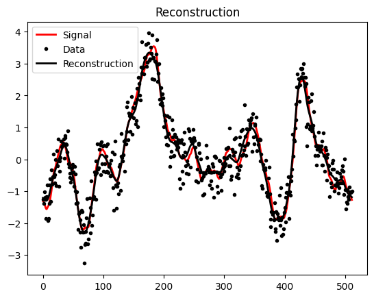
Results#

# Get signal data and reconstruction data
s_data = HT(sh).val
m_data = HT(m).val
d_data = d.val

plt.plot(s_data, 'r', label="Signal", linewidth=2)
plt.plot(d_data, 'k.', label="Data")
plt.plot(m_data, 'k', label="Reconstruction",linewidth=2)
plt.title("Reconstruction")
plt.legend()
plt.show()

png

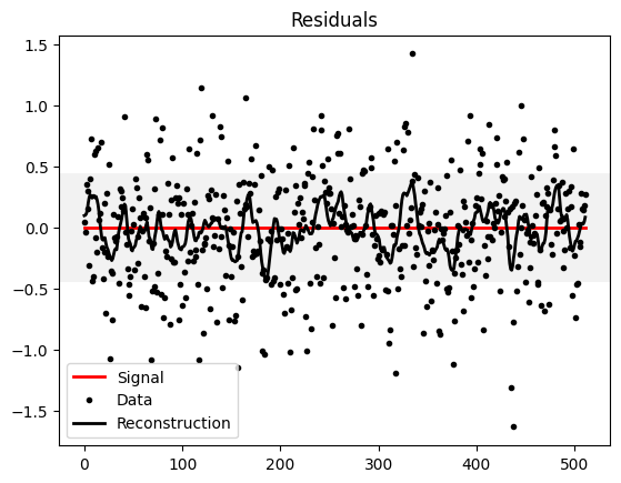
plt.plot(s_data - s_data, 'r', label="Signal", linewidth=2)
plt.plot(d_data - s_data, 'k.', label="Data")
plt.plot(m_data - s_data, 'k', label="Reconstruction",linewidth=2)
plt.axhspan(-noise_amplitude,noise_amplitude, facecolor='0.9', alpha=.5)
plt.title("Residuals")
plt.legend()
plt.show()

png

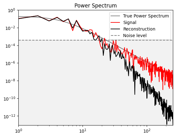
Power Spectrum#

s_power_data = ift.power_analyze(sh).val
m_power_data = ift.power_analyze(m).val
plt.loglog()
plt.xlim(1, int(N_pixels/2))
ymin = min(m_power_data)
plt.ylim(ymin, 1)
xs = np.arange(1,int(N_pixels/2),.1)
plt.plot(xs, pow_spec(xs), label="True Power Spectrum", color='k',alpha=0.5)
plt.plot(s_power_data, 'r', label="Signal")
plt.plot(m_power_data, 'k', label="Reconstruction")
plt.axhline(noise_amplitude**2 / N_pixels, color="k", linestyle='--', label="Noise level", alpha=.5)
plt.axhspan(noise_amplitude**2 / N_pixels, ymin, facecolor='0.9', alpha=.5)
plt.title("Power Spectrum")
plt.legend()
plt.show()

png

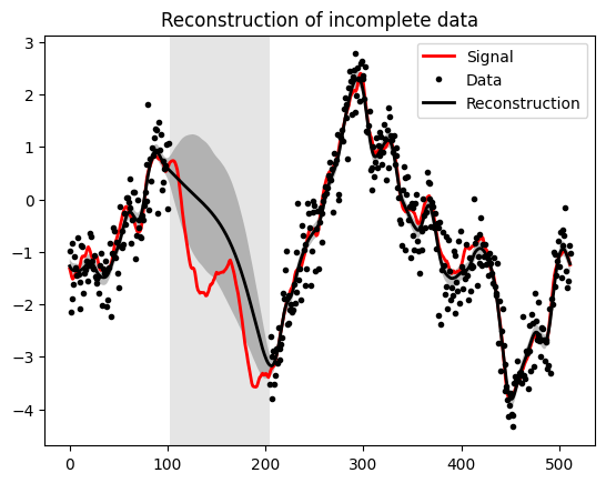
Wiener Filter on Incomplete Data#

# Operators
Sh = ift.create_power_operator(h_space, power_spectrum=pow_spec, sampling_dtype=float)
N = ift.ScalingOperator(s_space, noise_amplitude**2, sampling_dtype=float)
# R is defined below

# Fields
sh = Sh.draw_sample()
s = HT(sh)
n = ift.Field.from_random(domain=s_space, random_type='normal',
                      std=noise_amplitude, mean=0)

Partially Lose Data#

l = int(N_pixels * 0.2)
h = int(N_pixels * 0.2 * 2)

mask = np.full(s_space.shape, 1.)
mask[l:h] = 0
mask = ift.Field.from_raw(s_space, mask)

R = ift.DiagonalOperator(mask) @ HT
n = n.val_rw()
n[l:h] = 0
n = ift.Field.from_raw(s_space, n)

d = R(sh) + n

curv = Curvature(R=R, N=N, Sh=Sh)
D = curv.inverse
j = R.adjoint_times(N.inverse_times(d))
m = D(j)

Compute Uncertainty#

m_mean, m_var = ift.probe_with_posterior_samples(curv, HT, 200, np.float64)

Get data#

# Get signal data and reconstruction data
s_data = s.val
m_data = HT(m).val
m_var_data = m_var.val
uncertainty = np.sqrt(m_var_data)
d_data = d.val_rw()

# Set lost data to NaN for proper plotting
d_data[d_data == 0] = np.nan

plt.axvspan(l, h, facecolor='0.8',alpha=0.5)
plt.fill_between(range(N_pixels), m_data - uncertainty, m_data + uncertainty, facecolor='0.5', alpha=0.5)
plt.plot(s_data, 'r', label="Signal", alpha=1, linewidth=2)
plt.plot(d_data, 'k.', label="Data")
plt.plot(m_data, 'k', label="Reconstruction", linewidth=2)
plt.title("Reconstruction of incomplete data")
plt.legend()

<matplotlib.legend.Legend at 0x7ff34868b350>

png

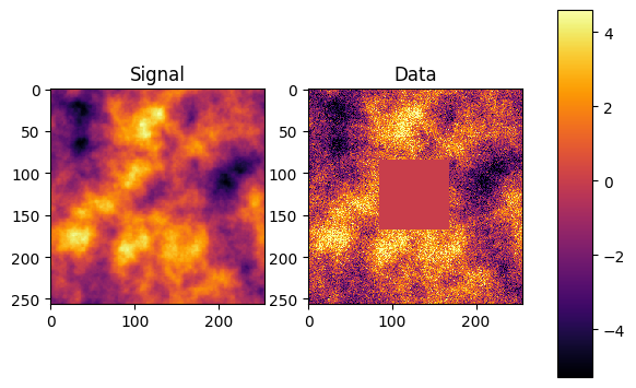
Wiener filter on two-dimensional field#

N_pixels = 256      # Number of pixels
sigma2 = 2.         # Noise variance

def pow_spec(k):
    P0, k0, gamma = [.2, 2, 4]
    return P0 * (1. + (k/k0)**2)**(-gamma/2)

s_space = ift.RGSpace([N_pixels, N_pixels])

h_space = s_space.get_default_codomain()
HT = ift.HarmonicTransformOperator(h_space,s_space)

# Operators
Sh = ift.create_power_operator(h_space, power_spectrum=pow_spec, sampling_dtype=float)
N = ift.ScalingOperator(s_space, sigma2, sampling_dtype=float)

# Fields and data
sh = Sh.draw_sample()
n = ift.Field.from_random(domain=s_space, random_type='normal',
                      std=np.sqrt(sigma2), mean=0)

# Lose some data

l = int(N_pixels * 0.33)
h = int(N_pixels * 0.33 * 2)

mask = np.full(s_space.shape, 1.)
mask[l:h,l:h] = 0.
mask = ift.Field.from_raw(s_space, mask)

R = ift.DiagonalOperator(mask)(HT)
n = n.val_rw()
n[l:h, l:h] = 0
n = ift.Field.from_raw(s_space, n)
curv = Curvature(R=R, N=N, Sh=Sh)
D = curv.inverse

d = R(sh) + n
j = R.adjoint_times(N.inverse_times(d))

# Run Wiener filter
m = D(j)

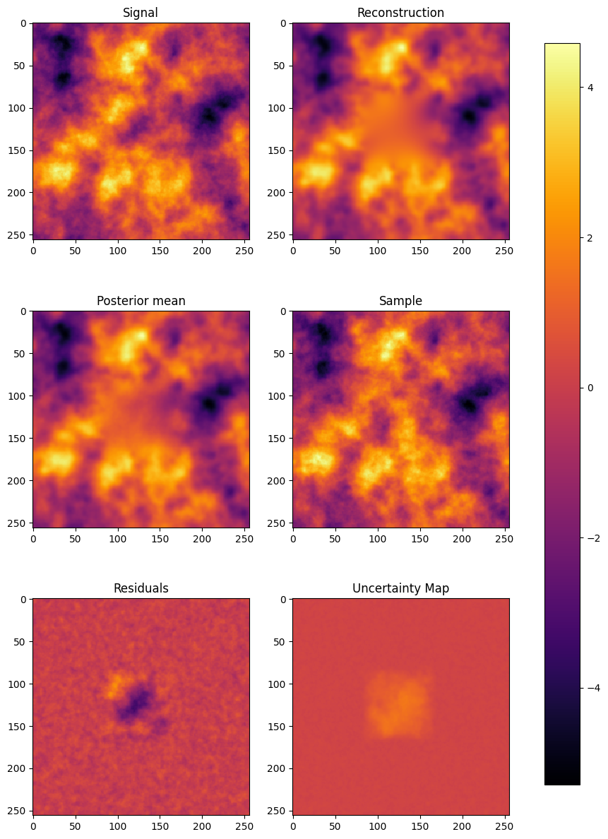
# Uncertainty
m_mean, m_var = ift.probe_with_posterior_samples(curv, HT, 20, np.float64)

# Get data
s_data = HT(sh).val
m_data = HT(m).val
m_var_data = m_var.val
d_data = d.val
uncertainty = np.sqrt(np.abs(m_var_data))

cmap = ['magma', 'inferno', 'plasma', 'viridis'][1]

mi = np.min(s_data)
ma = np.max(s_data)

fig, axes = plt.subplots(1, 2)

data = [s_data, d_data]
caption = ["Signal", "Data"]

for ax in axes.flat:
    im = ax.imshow(data.pop(0), interpolation='nearest', cmap=cmap, vmin=mi,
                   vmax=ma)
    ax.set_title(caption.pop(0))

fig.subplots_adjust(right=0.8)
cbar_ax = fig.add_axes([0.85, 0.15, 0.05, 0.7])
fig.colorbar(im, cax=cbar_ax)

<matplotlib.colorbar.Colorbar at 0x7ff348a13ed0>

png

mi = np.min(s_data)
ma = np.max(s_data)

fig, axes = plt.subplots(3, 2, figsize=(10, 15))
sample = HT(curv.draw_sample(from_inverse=True)+m).val
post_mean = (m_mean + HT(m)).val

data = [s_data, m_data, post_mean, sample, s_data - m_data, uncertainty]
caption = ["Signal", "Reconstruction", "Posterior mean", "Sample", "Residuals", "Uncertainty Map"]

for ax in axes.flat:
    im = ax.imshow(data.pop(0), interpolation='nearest', cmap=cmap, vmin=mi, vmax=ma)
    ax.set_title(caption.pop(0))

fig.subplots_adjust(right=0.8)
cbar_ax = fig.add_axes([.85, 0.15, 0.05, 0.7])
fig.colorbar(im, cax=cbar_ax)

<matplotlib.colorbar.Colorbar at 0x7ff344a0c610>

png

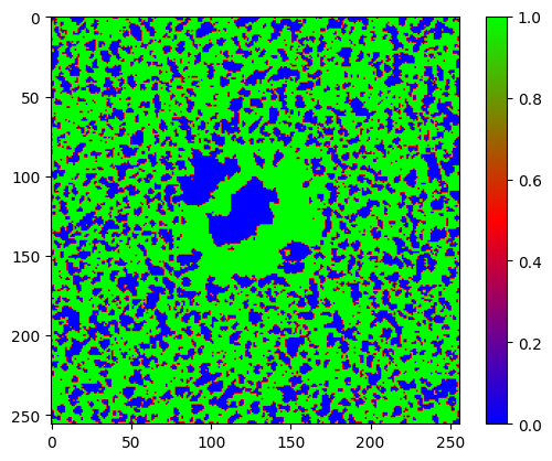
Is the uncertainty map reliable?#

precise = (np.abs(s_data-m_data) < uncertainty)
print("Error within uncertainty map bounds: " + str(np.sum(precise) * 100 / N_pixels**2) + "%")

plt.imshow(precise.astype(float), cmap="brg")
plt.colorbar()

Error within uncertainty map bounds: 67.71392822265625%

<matplotlib.colorbar.Colorbar at 0x7ff34421f250>

png